Decay Linear Discriminant Analysis#
Documentation for iq_readout.two_state_classifiers.DecayLinearClassifier
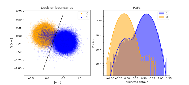
The PDFs are derived in Improved quantum error correction using soft information by Pattison et al. (arxiv pdf). In this classifier, the \(p(\vec{z}|0)\) is a mixture of Gaussians to handle state preparation errors in the readout calibration data.
Characteristics#
2-state classifier for 2D data
Uses max-likelihood classification
Decision boundary is a straight line (hence linear)
Assumes that the integration weights of the readout traces (output voltage as a function of time) are constant
Assumes that the Gaussian distributions present in \(p(\vec{z}|i)\) share the same covariance matrix \(\Sigma=\mathrm{diag}(\sigma^2, \sigma^2)\) and means \(\vec{\mu}_0, \vec{\mu}_1\)
and
with \(\vec{z} = z_{\perp} \hat{e}_{\perp} + z_{\parallel} \hat{e}_{\parallel}\), \(\hat{e}_{\parallel} = (\vec{\mu}_1 - \vec{\mu}_0) / |\vec{\mu}_1 - \vec{\mu}_0|\), \(\hat{e}_{\perp} \perp \hat{e}_{\parallel}\),
a 2D Gaussian with covariance matrix \(\Sigma=\mathrm{diag}(\sigma^2, \sigma^2)\),
a 1D Gaussian,
and \(\tilde{T}_1 = T_1 / t_M\) the normalized amplitude decay time with respect to the measurement time.
Example#
Max-likelihood classifier#
Given \(\vec{z}\), a max-likelihood classifier outputs the class \(c\) that has larger probability (given \(\vec{z}\)), i.e. \(c\) such that \(p(c|\vec{z}) \geq p(j|\vec{z}) \;\forall j \neq c\). These probabilities are calculated using Bayes’ theorem and the probabilities of the qubit being in state \(j\), \(p(j)\). By default, it uses \(p(j)=1/2\), where \(p(c|\vec{z}) \geq p(j|\vec{z}) \forall j \neq c\) is equivalent to \(p(\vec{z}|c) \geq p(\vec{z}|j) \forall j \neq c\).
Linearity#
The decision boundary for (2-state) max-likelihood classifiers is given by the (parametrized) curve \(\vec{d}(t)\) that fulfills \(p(0|\vec{d}) = p(1|\vec{d}) \;\forall t\). As the PDFs \(p(\vec{z}|i)\) are symmetric with respect to \(z_{\parallel}\), the decision boundary must also be symmetric. Moreover, because the contribution of \(z_{\perp}\) to \(p(\vec{z}|i)\) is the same for both \(i=0\) and \(i=1\) (i.e. \(\tilde{N}_1(z_{\perp}; \vec{\mu}_{1,\perp}, \sigma)\) with \(\vec{\mu}_{1,\perp}=\vec{\mu}_{0,\perp}\)), then the decision boundary is of the form \(f(z_{\parallel}) = g(z_{\parallel}) \\;\forall z_{\perp}\). Therefore the decision boundary is a straight line along the direction of \(\hat{e}_{\perp}\) that crosses the point in the \(\hat{e}_{\parallel}\)-axis that fulfills \(f(z_{\parallel}) = g(z_{\parallel})\).
Notes on the algorithm#
The algorithm for setting up the classifier from the readout calibraton data is based on fitting the PDFs to the histograms of the data. If the data does not fulfill the assumptions described above, the classifier may not be the optimal one (in the sense of optimal Bayes classifier and minimal Bayes error rate). For example, the linear classifier from sklearn may lead to a higher readout fidelity (even though they are both linear classifiers) because its decision boundary is found by minimizing the classification error.
As the classifier is linear, the data can be projected to the axis orthogonal to the decision boundary. The projection axis corresponds to the line with direction \(\vec{\mu}_1 - \vec{\mu}_0\) that crosses these two means. The direction is chosen this way to have the blob from state 0 on the left and the blob from state 1 on the right. The projection axis can be estimated from the means of the data for each class \(c\), \(\{\vec{z}^{(i)}_c\}_i\), given by
because \(\vec{\mu}_1 - \vec{\mu}_0 \propto \vec{\nu}_1 - \vec{\nu}_0\). The justification follows the same used in the linearity section.
The algorithm uses the following tricks:
work with projects the data (to have more samples in each bin of the histogram)
combine \(\vec{z}_c\) from both classes to extract the means and standard deviation (to have more samples in each bin of the histogram). Note: the parameters \(\theta_c\) are extracted from each \(\vec{z}_c\)
The algorithm can give \(p(z_{\parallel}|i)\) with \(z_{\parallel}\) the projection of \(\vec{z}\) or \(p(\vec{z}|i)\). Note that the two pdfs are related, i.e. \(p(z_{\parallel}|0) / p(z_{\parallel}|1) = p(\vec{z}|0) / p(\vec{z}|1)\). The explanation can be found in classifiers/gmlda:Gaussian-Mixture Linear Discriminant Analysis.