Gaussian-Mixture Linear Discriminant Analysis#
Documentation for iq_readout.two_state_classifiers.GaussMixLinearClassifier
Characteristics#
2-state classifier for 2D data
Uses max-likelihood classification
Decision boundary is a straight line (hence linear)
Assumes that the classes follow a Gaussian mixture that share the same covariance matrix \(\Sigma=\mathrm{diag}(\sigma^2, \sigma^2)\) and means \(\vec{\mu}_0, \vec{\mu}_1\), i.e.
and
with
a 2D multivariate Gaussian with covariance matrix \(\Sigma=\mathrm{diag}(\sigma^2, \sigma^2)\).
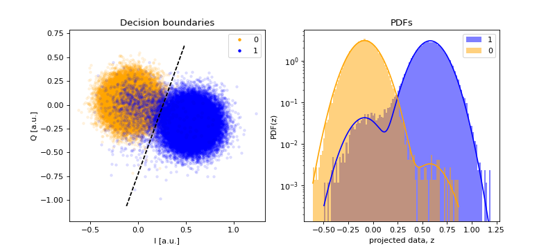
Example#
Max-likelihood classifier#
Given \(\vec{z}\), a max-likelihood classifier outputs the class \(c\) that has larger probability (given \(\vec{z}\)), i.e. \(c\) such that \(p(c|\vec{z}) \geq p(j|\vec{z}) \;\forall j \neq c\). These probabilities are calculated using Bayes’ theorem and the probabilities of the qubit being in state \(j\), \(p(j)\). By default, it uses \(p(j)=1/2\), where \(p(c|\vec{z}) \geq p(j|\vec{z}) \forall j \neq c\) is equivalent to \(p(\vec{z}|c) \geq p(\vec{z}|j) \forall j \neq c\).
Linearity#
The decision boundary for (2-state) max-likelihood classifiers is given by the (parametrized) curve \(\vec{d}(t)\) that fulfills \(p(0|\vec{d}) = p(1|\vec{d}) \;\forall t\). As the PDFs \(p(\vec{z}|i)\) are symmetric with respect to \(z_{\parallel}\), the decision boundary must also be symmetric. Moreover, because the contribution of \(z_{\perp}\) to \(p(\vec{z}|i)\) is the same for both \(i=0\) and \(i=1\) (i.e. \(\tilde{N}_1(z_{\perp}; \vec{\mu}_{1,\perp}, \sigma)\) with \(\vec{\mu}_{1,\perp}=\vec{\mu}_{0,\perp}\)), then the decision boundary is of the form \(f(z_{\parallel}) = g(z_{\parallel}) \\;\forall z_{\perp}\). Therefore the decision boundary is a straight line along the direction of \(\hat{e}_{\perp}\) that crosses the point in the \(\hat{e}_{\parallel}\)-axis that fulfills \(f(z_{\parallel}) = g(z_{\parallel})\).
The expression for \(\vec{d}(t)\) can be found as follows. Firstly, we make use of the Bayes’ theorem and substitue \(p(\vec{z}|i)\) for this classifier to get
with \(c_0 = \sin^2(\theta_0)\) and \(b_0 = \sin^2(\theta_1)\). By multiplying the expression by \(\exp(+|\vec{d} - \vec{\mu}_0|^2 / 2\sigma^2)\) and rearraging terms, we can write
After taking the logarithm and using \(|\vec{a}|^2 - |\vec{b}|^2 = (\vec{a} - \vec{b})(\vec{a} + \vec{b})\), we obtain the linear equation
with solution
with \(t \in \mathbb{R}\) and \(\vec{\mu}_{\perp}\) the vector perpendicular to \(\vec{\mu}_0 - \vec{\mu}_1\). This curve is a line that is perpendicular with the axis defined by the two blobs in the IQ plane. In the particular case \(p(0) = 1/2\), then \(P=1\) and thus the line is in the middle of the two blobs.
Notes on the algorithm#
The algorithm for setting up the classifier from the readout calibraton data is based on fitting the PDFs to the histograms of the data. If the data does not fulfill the assumptions described above, the classifier may not be the optimal one (in the sense of optimal Bayes classifier and minimal Bayes error rate). For example, the linear classifier from sklearn may lead to a higher readout fidelity (even though they are both linear classifiers) because its decision boundary is found by minimizing the classification error.
As the classifier is linear, the data can be projected to the axis orthogonal to the decision boundary. The projection axis corresponds to the line with direction \(\vec{\mu}_1 - \vec{\mu}_0\) that crosses these two means. The direction is chosen this way to have the blob from state 0 on the left and the blob from state 1 on the right. The projection axis can be estimated from the means of the data for each class \(c\), \(\{\vec{z}^{(i)}_c\}_i\), given by
because \(\vec{\mu}_1 - \vec{\mu}_0 \propto \vec{\nu}_1 - \vec{\nu}_0\). The justification is that, given \(\vec{z}_c \sim p(\vec{z}|c)\), the estimator of the mean is \(\vec{\nu}_c = \sin^2(\theta_c) \vec{\mu}_0 + \cos^2(\theta_c) \vec{\mu}_1\), thus \(\vec{\nu}_1 - \vec{\nu}_0 = (\sin^2(\theta_1) - \sin^2(\theta_0)) (\vec{\mu}_1 - \vec{\mu}_0)\).
The algorithm uses the following tricks:
work with projected data (to have more samples in each bin of the histogram)
combine \(\vec{z}_c\) from both classes to extract the means and standard deviation (to have more samples in each bin of the histogram). Note: the parameters \(\theta_c\) are extracted from each \(\vec{z}_c\)
The algorithm can give \(p(z_{\parallel}|i)\) with \(z_{\parallel}\) the projection of \(\vec{z}\) or \(p(\vec{z}|i)\). Note that the two pdfs are related, i.e. \(p(z_{\parallel}|0) / p(z_{\parallel}|1) = p(\vec{z}|0) / p(\vec{z}|1)\). The explanation uses the coordinate system of the projection axis and its perpendicular, labelled \(\vec{z} = z_{\parallel} \hat{e}_{\parallel} +z_{\perp}\hat{e}_{\perp}\), which gives
because \(\vec{\mu}_{0,\perp} = \vec{\mu}_{1,\perp}\) and the terms cancel each other. We then just need to use that
leading to \(p(z_{\parallel}|0) / p(z_{\parallel}|1) = p(\vec{z}|0) / p(\vec{z}|1)\).