Max-Fidelity Linear Discriminant Analysis#
Documentation for iq_readout.two_state_classifiers.MaxFidLinearClassifier
Characteristics#
2-state classifier for 2D data
Uses threshold to classify (projected) 2D data
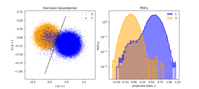
Decision boundary is a straight line (hence linear)
Does not assume any probability density function for the 2D data, thus
the PDFs will correspond to the histograms of the calibration data
the accuracy in the threshold is limited by the bin separation of the histogram of the calibration data
Example#
Threshold classifier#
The threshold classifiers are two-state linear classifiers that use a threshold line (hence linear) to divide the 2D plane into two regions (hence two-state classifier). Given a threshold \(z_{thr}\) and a projection function \(\vec{z} \rightarrow z_{\parallel}=\vec{z}\cdot \hat{e}_{\parallel}\), it outputs 0 if \(z_{\parallel} \leq z_{thr}\) and 1 otherwise.
Note: the threshold can be updated based on the prior probabilities of the classes, but it requires some computation
Linearity#
The linearity of this classifier comes from its definition, as the decision boundary is a line perpendicular to \(\hat{e}_{\parallel}\) that crosses the point \(\vec{A} = z_{thr}\hat{e}_{\parallel}\).
Maximum fidelity in a threshold classifier#
The assignment infidelity \(\epsilon\) is defined as \(\epsilon = (p(m=0|s=1) + p(m=1|s=0))/2\), where \(p(m|s)\) is the probability of measuring \(m\) given that the qubit was in state \(s\). Note that we have assumed that the probability of seeing state 0 and 1 are the same (i.e. p(s=0)=p(s=1)=1/2), but it can be generalized to any \(p(s)\) using \(\epsilon = p(m=1|s=0)p(s=0) + p(m=0|s=1)p(s=1)\). Given the cumulative density functions \(CDF(z_{\parallel}|s)\), we can rewrite the assingment infidelity as
because the probability of incorrectly assigning \(m=0\) to state \(s=1\) is the probability that the projected data is less than the threshold, and equivalently for the other case. Note that we have assumed that (1) the 0 blob is on the left of the 1 blob in the projected axis, and (2) the density functions “behave as expected”, meaning that \(CDF(z_{\parallel}|0) \geq CDF(z_{\parallel}|1) \;\forall z_{\parallel}\). This last assumption can be broken if the PDFs exhibit more than one maximum.
The threshold that maximizes the assingment fidelity \(F = 1 - \epsilon\) (i.e. minimizes the assignment infidelity) is given by the point that maximizes the distance between the cumulative density functions,
where we have omited the constants and factors as we are only interested in the \(\mathrm{argmax}\), not the \(\mathrm{max}\) value. In the general case where the priors are not equal, we have
Notes on the algorithm#
As the classifier is linear, the data can be projected to the axis orthogonal to the decision boundary. The projection axis corresponds to the line with direction \(\vec{\mu}_1 - \vec{\mu}_0\) that crosses these two means. The direction is chosen this way to have the blob from state 0 on the left and the blob from state 1 on the right. The projection axis can be estimated from the means of the data for each class \(c\), \(\{\vec{z}^{(i)}_c\}_i\), given by
because \(\vec{\mu}_1 - \vec{\mu}_0 \propto \vec{\nu}_1 - \vec{\nu}_0\). The justification is that, given \(\vec{z}_c \sim p(\vec{z}|c)\), the estimator of the mean is \(\vec{\nu}_c = \sin^2(\theta_c) \vec{\mu}_0 + \cos^2(\theta_c) \vec{\mu}_1\), thus \(\vec{\nu}_1 - \vec{\nu}_0 = (\sin^2(\theta_1) - \sin^2(\theta_0)) (\vec{\mu}_1 - \vec{\mu}_0)\).
The algorithm uses the following tricks:
work with projected data (to have more samples in each bin of the histogram)